
|
| THE ELECTRONIC JOURNAL OF COMBINATORICS (ed. June 2005), DS #5. |
An n-Venn diagram C = {C1,...,Cn} may be regarded as a graph in two ways. The diagram itself can be thought of as an edge-colored plane5 graph V(C) whose vertices correspond to intersections of curves, and whose edges correspond to the segments of curves between intersections. Edges are colored according to the curve to which they belong. Following Chilakamarri, Hamburger, and Pippert [CHP], we overload the term and call this graph the Venn diagram. In an unlabelled Venn diagram we ignore the edge labels. As an example, the three circle Venn diagram has 6 vertices (corresponding to the 6 intersections) and 12 edges. Recall Euler's formula f = e - v + 2 relating the number of faces, edges, and vertices of a graph embedded in the plane. Assuming that no three curves intersect at a common point (i.e., a simple Venn diagram), we have e = 2v. By definition the number of faces is f = 2n. It thus follows that v = 2n - 2 and e = 2n+1 - 4 for simple Venn diagrams.
Two curves can meet at a point transversally or not, depending on whether the two curves cross. A moment's reflection will convince you that the curves in a simple Venn diagram must meet transversally. More generally, at any point of intersection in a Venn diagram, there must be at least two curves that meet transversally.
With each Venn diagram, C, we may associate another plane graph called the Venn dual, and denoted D(C), which is the planar dual of the Venn diagram. (Some authors use the term "Venn graph" to refer to the dual.) Its vertices are the connected open regions (faces) of V(C). Two vertices are connected by an edge if they share a common boundary. By default the edges are colored (by the color of the corresponding edge in the Venn diagram). At times it is also useful to label the vertices with a length-n bitstring consisting of 0s and 1s; if the curves are labelled 1 to n then we set bit i to 1 if the vertex is enclosed by curve i, 0 otherwise. Labels of adjacent vertices differ in exactly one bit position as one curve in the Venn diagram is crossed by one edge in the Venn dual. For example, the Venn dual of the three circle Venn diagram is a planar embedding of the 3-cube, Q3. Clearly, every n-Venn dual is a planar spanning subgraph of the n-cube, Qn. If C is a simple Venn diagram, then every face of D(C) is a quadrilateral, and thus D(C) is a maximal bipartite8 planar graph.
On the other hand, a Venn diagram may be embedded in the sphere via stereographic projection. (Consider the standard tennis ball; it is the stereographic projection of Edwards' general construction for n = 4.) Sometimes it is more natural to look at Venn diagrams as being embedded on the sphere. Two Venn diagrams are in the same class if they can be projected to the same spherical Venn diagram.
When considering non-simple Venn diagrams there is another elementary operation that can sometimes be applied to one diagram to get another.
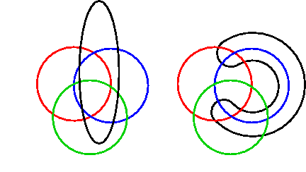
Definition: A vertex traversal of a vertex v in a Venn diagram is a circular sequence C0, C1, ..., Cm of the curves adjacent to v, when read in a clockwise rotation around v. A vertex is said to be separable if its vertex traversal has the property that for some i, there is a j such that the intersection of A = {Ci, Ci+1,...,Cj-1} and B = {Cj, Cj+1,...,Ci-1} consists of one curve, say C, and in addition, |A| > 2 and |B| > 2. In the example below the sets A and B are A = { red, green, black, red, green} and B = {blue, yellow, black, blue, yellow}, and the black curve is the curve C. A Venn diagram is said to be rigid if it has no separable vertices. The figures below illustrate the operation of splitting a separable vertex; unsplitting is defined as the inverse operation.
| <===> |
|
|
An example of a separable vertex. This is a Venn diagram |
iff |
Splitting the separable vertex. this is a Venn diagram |
Simple diagrams are in many ways the most pleasing of Venn diagrams. Rigid Venn diagrams are interesting because in the equivalence class of diagrams under splitting and unsplitting of vertices, they are the ones closest to being simple.
This page shows an example of creating a simple symmetric diagram from a non-simple diagram by splitting vertices in a symmetric fashion.
The precise number of Venn diagrams and Venn classes has been determined by Chilakamarri, Hamburger and Pippert [CHP96b, HP97, CHP00] for n = 1,2,3, and for simple diagrams and classes if n = 4 and 5. Clearly, for n = 1,2 there is only one diagram.
For n = 3 there are six distinct Venn classes and fourteen distinct Venn diagrams. Only one of the diagrams is simple (Class 6).
Note that classes 2 and 3 are equivalent but not isomorphic, as are diagrams #3.3 & #3.6 (and #3.4 & #3.5). Diagram #3.3 appears also in [ES] (showing that it is a convex12 diagram). The diagrams in Class 2 have the property that each pair of curves at a point of intersection meet transversally; the diagrams of Class 3 do not have this property. Aside from the simple diagram of Class 6, only Class 2 is rigid; the other classes are non-rigid.
For n = 4 there are two distinct simple Venn diagrams and one distinct simple Venn class (this was first observed by Grünbaum [Gr92a,p.8] and proven in [CHP96b]). Drawings of these two are shown in Figures 4 (a) and (b) in [Gr92a,p.7], and are reproduced here:
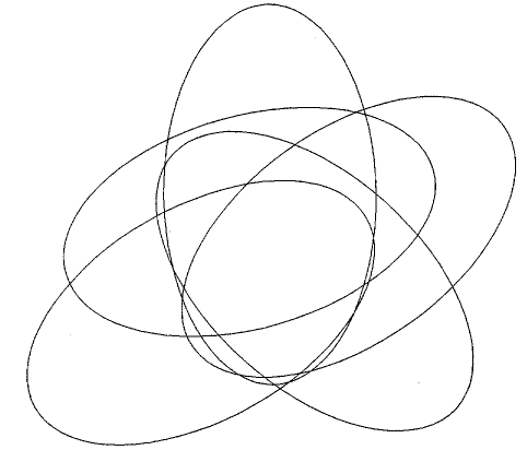
For n = 5, there are 11 distinct, reducible, simple Venn classes and 12 distinct, reducible, simple Venn diagrams. Drawings of these may be found in [HP97]. There are 8 distinct simple, irreducible Venn classes ([CHP00]). Five of them have one convex drawing in the plane (and four of these were discovered by Grünbaum). All five can be drawn with five congruent ellipses. Thus, in total, there are 19 simple Venn classes for n = 5.
In proving these results several theorems of independent interest were proven:
Theorem H1. A simple Venn diagram for n > 2 is 3-connected.
A theorem of Whitney [Wh] states that a plane embedding of a 3-connected planar graph is unique, once the outer face has been identified. Thus, to determine whether two diagrams are in the same class, we need only try all possible embeddings of one of them with each of its faces as the outer region and observe whether any of these embeddings is isomorphic to the other diagram.
Theorem H2. A simple Venn dual graph for n > 2 is 3-connected.
Theorem H3. No two edges in a face in a Venn diagram belong to the same curve.
The total number of Venn diagrams for n = 6 is not known. As part of his search for 6-Venn triangles, Carroll [Car99] reports that there are 1833 non-isomorphic simple monotone 6-Venn diagrams with the additional property that there are no more than 6 crossings between any pair of curves.
A Venn diagram is reducible if the removal of one of its n curves results in a Venn diagram with n-1 curves. The two general constructions, by their nature, both yield reducible diagrams. A Venn diagram that is not reducible is irreducible. The symmetric ellipse diagram shown below is irreducible; this page shows why. For a long time it was not known whether a reducible Venn diagram whose curves are ellipses existed or not; such a diagram was discovered by Hamburger and Pippert [HP00] and is shown below.
A n-Venn diagram C is extendible if there is a curve that can be added to it to make an (n+1)-Venn diagram, C'. Diagram C' is said to be an extension of C. Winkler [Wi] makes the following two observations:
Theorem W1. For n > 1, a simple n-Venn diagram C is extendible to a simple (n+1)-Venn diagram if and only if its Venn dual D(C) is Hamiltonian.
Theorem W2. If the n-Venn diagram C is an extension of an (n-1)-Venn diagram, then C is extendible to an (n+1)-Venn diagram.
To prove the latter theorem, let B be the diagram whose extension is C. By Theorem W1, The curve H added to B to get C corresponds to a Hamiltonian cycle in D(B). In D(C), curve H becomes the prism4, P, of a cycle of length 2n. Since the prism of a cycle is Hamiltonian, C is extendible.
Edwards' general construction is a manifestation of this proof of Theorem W2, where the Hamilton cycle in P is the one that alternates back and forth between the two copies of the cycle, two vertices at a time from each cycle. Venn's general construction is related but different since it uses non-prism edges (example).
The proof of [CHP96a] introduces the radual graph, R(C) of the Venn diagram, which, for an arbitrary plane graph, is the union of the radial graph and the dual graph (Ore [Or] has more information on the radial and dual graphs). A simple example, using Venn diagram #3.4 is shown here. The strategy of their proof is first to show that R(C) is a simple triangulation without separating triangles and then invoke a theorem of Whitney [Wh] that any such graph is Hamiltonian. It is then easy to see that the Hamilton cycle in the radual graph can be used as the additional curve. This sufficient condition is also necessary as stated in this analogue of Theorem W1.
Theorem CHP1. For n > 1, a n-Venn diagram C is extendible to a (n+1)-Venn diagram if and only if its radual graph R(C) is Hamiltonian.
| In a simple Venn diagram the number of vertices is exactly 2n-2. For non-simple Venn diagrams this number can be reduced, but a lower bound of ceiling[ (2n-2)/(n-1) ] is readily derived from Euler's relation and the fact that at most n curves can intersect at a point. Diagrams achieving this lower bound are known for n = 2 to 7, and are said to be minimum. For n=3 diagrams #3.1 and #3.2 achieve this lower bound. For n=4 the diagram shown here (discovered in collaboration with Peter Hamburger) achieves the lower bound. See examples for n=5 (from [BR]), and examples for n=7 (discovered in collaboration with Stirling Chow). |
|
A Venn diagram is monotone if, for 0 < k < n, every k-region is adjacent to both a (k-1)-region and a (k+1)-region. The general construction of Edwards is monotone; the general construction of Venn is not. Examples of monotone and non-monotone Venn diagrams may be found on the Symmetric Venn Diagrams page. The 3-Venn diagrams 3.12 and 3.13, both in the same class, show that monotonicity is a property of Venn diagrams and not Venn classes, as 3.12 is monotone and 3.13 is not. In a monotone Venn diagram the k-regions, for any 0 < k < n, form a "cycle", in the sense that every k-region touches exactly two others, and they are connected together in a cycle under this relation [BR].
We can view monotonicity in another order-theoretic way. The Venn dual graph, D(C), defined above, could have been defined as a directed acyclic graph, with the direction indicating whether one vertex is a subset of another. Let's call this the directed Venn dual graph. The directed Venn dual is a spanning subgraph of the Hasse diagram (regarded as a directed graph) of the Boolean lattice. As shown in [BGR], a Venn diagram is monotone if and only if the directed Venn dual graph has a unique maximum element (sink) and a unique minimum element (source).
Bultena and Ruskey [BR] determined Mn, the least number of vertices in a monotone n-Venn diagram.
Theorem B. Mn = C( n, n/2 ), where C denotes a binomial coefficient1.
They also gave an inductive construction to show that monotone Venn diagrams that achieve this bound exist for all n > 1. A constructive proof with a different motivation is given in [GKS].
The first part of this section is more "geometric" than "graph theoretic". We introduce congruent Venn diagrams here because the examples are used to illustrate graph theoretic definitions.
The general constructions of Venn and Edwards outlined on the "What is a Venn Diagram?" page do not share a nice property of the first two figures on the same page (made from circles and triangles), namely, that they are constructed from congruent2 curves. Grünbaum [Gr92b] defines a Venn diagram to be nice if it is made from congruent curves, but we'll prefer to call them congruent Venn diagrams. The first such diagrams were constructed by Grünbaum in the seminal paper [Gr75]. In [Gr92b] he discussed examples of congruent diagrams for up to 8 curves; many symmetric examples can be found on the Symmetric Venn Diagrams page.
 Hamburger and Pippert [HP97]
proved that there are simple reducible Venn diagrams with
5 congruent ellipses, in spite of the fact that Venn had stated
that there are no such diagrams.
In fact, there are two of them, but they are in the same class: one
of their diagrams is shown to to the right.
Hamburger and Pippert [HP97]
proved that there are simple reducible Venn diagrams with
5 congruent ellipses, in spite of the fact that Venn had stated
that there are no such diagrams.
In fact, there are two of them, but they are in the same class: one
of their diagrams is shown to to the right.
Below we show a redrawing of Grünbaum's beautiful congruent Venn diagram (from [Gr75]) made from 5 congruent ellipses which also has a rotational symmetry. The diagram on the left labels each region with the labels of all ellipses that contain the region. On the right, the regions are colored according to the number of ellipses in which they are contained: white (the external region) = 0, yellow = 1, red = 2, blue = 3, green = 4, and black = 5. Note that the number of regions colored with a given color corresponds to the appropriate binomial coefficient: #(white) = #(black) = 1, #(yellow) = #(green) = 5, and #(red) = #(blue) = 10.
 |
 |
| 1 | 2 | 3 | 4 | 5 |
| 12 | 13 | 15 | 25 | 45 | 14 | 34 | 35 | 23 | 24 |
| 123 | 135 | 125 | 245 | 145 | 134 | 345 | 235 | 234 | 124 |
| 1234 | 1235 | 1245 | 1345 | 2345 |
Because of the symmetry of the diagram, these circular listings have the property that they remain invariant when acted on by the cyclic permutation (1 2 3 4 5). These listings are related to combinatorial Gray codes; since Gray codes have many connections with symmetric diagrams we describe them further on the Variants on Symmetry page in their own section.
|
| THE ELECTRONIC JOURNAL OF COMBINATORICS (ed. June 2005), DS #5. |